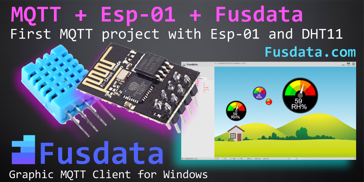
In this post we are going to explain step by step how to launch the first Iot Project with Esp-01 and Fusdata. Specifically, we are going to implement the example of Fusdata.com.ar website in which a DHT-11 sensor is used to monitor the relative humidity and temperatura inside a house.
Although the example is simple, we are going to develop it in an integral way so that concepts are useful for future Fusdata projects.
We are going to use:
A Esp-01 module (Esp8266).
A DHT-11 Sensor.
The Fusdata MQTT client for Windows (fusdata.com.ar).
A public MQTT TCP Broker for testing.
Arduino IDE programming environment.
ESP8266WiFi.h library.
PubSubClient.h library.
DHT.h library.
Firmware is available here (https://fusdata.com.ar/en/support/).
Primer proyecto MQTT con Fusdata y Esp-01
En esta entrada vamos a explicar paso a paso como poner en marcha el primer proyecto Iot con Esp-01 y Fusdata. Concretamente vamos a implementar el ejemplo de la página web Fusdata.com.ar en la que se utiliza un sensor DHT-11 para monitorear humedad relativa y temperatura dentro de una vivienda.
Si bien el ejemplo es muy sencillo, vamos a desarrollarlo de manera integral para que los conceptos sean útiles también en futuros proyectos de Fusdata.
Vamos a utilizar:
Un módulo Esp-01 (Esp8266).
Sensor DHT-11.
El cliente MQTT Fusdata (fusdata.com.ar).
Un Broker MQTT TCP público para pruebas.
Entorno de programación Arduino IDE.
Librería ESP8266WiFi.h
Librería PubSubClient.h
Librería DHT.h
El firmware está disponible aquí (https://fusdata.com.ar/en/support/).
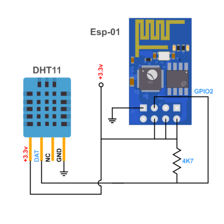
Electronic scheme
Esquema electrónico
For this example I have thought of using the GPI02 pin of the ESP-01 module because i want to leave the GPIO0, GPIO1 and GPIO3 pins available for future functions. I any case, you can use the pin you want just by modifying the firmware.
Para este ejemplo he pensado en utilizar el pin GPIO2 del módulo Esp-01 porque deseo dejar disponibles los pines GPIO0, GPIO1 y GPIO3 para futuras funciones. De todas maneras tu puedes utilizar el pin que quieras solo modificando el firmware.
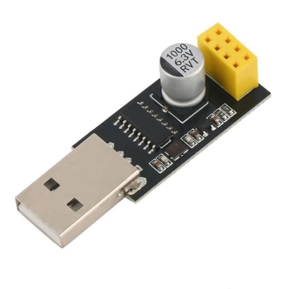
Although it is not the purpose of this tutorial to talk about how to program the ESP-01 module, I want to commnet on the excellent results this usb module has given me:
Aunque no es el propósito de este tutorial hablar sobre cómo programar el módulo Esp-01 quiero comentar que me ha dado excelente resultado este módulo usb:
When programming the module, I enable a jumper that connects the GND and GPI00 pins welded very carefully on the underside of the board. Then, to test the operation, I put the ESP-01 on a very simple board of my owan designed powered by 3.3V.
Al momento de la programación del módulo habilito un puente “jumper” que conecta los pines GND y GPIO0 soldado con mucho cuidado del lado de debajo de la placa. Luego para probar el funcionamiento, coloco el Esp-01 en una placa muy sencilla de mi propio diseño alimentado solo con 3.3V.
Firmware
The firmware that I provide you for downloading is called “Ernesto_1x.ino” and it is a simple program for Arduino Ide that performs all the mínimum and necessary functions to send the data from the sensor to the cloud using the MQTT protocol.
The first lines of the program show the following parameters to customize:
const char* ssid = “WFssid”; // Your WiFi name
const char* password = “WFpass”; // Your WiFi pass
const char* mqtt_server = “test.mosquitto.org”; // Your url MQTT Broker
const unsigned int mqtt_port = 1883; // MQTT Broker port
const char* topic_tx = “Ernesto/sub_tp”; // Topic Root/Sub-topical
const char* topic_rx = “Ernesto/A00001”; // Topic for subscribe Root/sender_id
const char* sender_id = “A00001”; // Device Sender ID
You can use a free MQTT Broker for testing, the following is the one I use:
test.mosquitto.org
broker.hivemq.com
public.mqtthq.com
broker.emqx.io
El firmware que he puesto para descarga se denomina “Ernesto_1x.ino” y es un sencillo programa para Arduino Ide que realiza todas las funciones mínimas y necesarias para lograr enviar los datos provenientes del sensor a la nube utilizando el protocolo MQTT.
Las primeras líneas del programa muestran los siguientes parámetros a personalizar:
const char* ssid = “WFssid”; // Your WiFi name
const char* password = “WFpass”; // Your WiFi pass
const char* mqtt_server = “test.mosquitto.org”; // Your url MQTT Broker
const unsigned int mqtt_port = 1883; // MQTT Broker port
const char* topic_tx = “Ernesto/sub_tp”; // Topic Root/Sub-topical
const char* topic_rx = “Ernesto/A00001”; // Topic for subscribe Root/sender_id
const char* sender_id = “A00001”; // Device Sender ID
Puedes utilizar un Broker MQTT gratuito para pruebas, éstos que pongo a continuación son los que yo utilizo:
test.mosquitto.org
broker.hivemq.com
public.mqtthq.com
broker.emqx.io
With any of them we can connect through port 1883 since the protocol will be normal TCP without TLS security.
Access to the MQTT Broker will be anonymous so the “User” and “Password” credentials will not be needed.
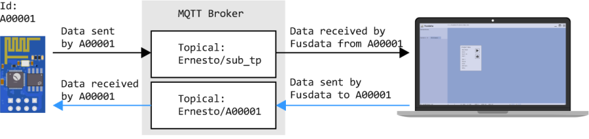
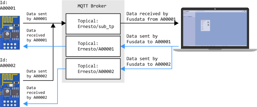
It is very important to grasp the meaning of the concept “Root”. It is under this topic that your entire MQTT data transmission system is organized.
I have chosen “Ernesto”as a root topic.
Then our device that we will call “sender” must have a unique name or identification called “sender_ID”, which is a small string of characters between ascii (33 and ascii(122). It is recommended between 4 and 8 characters and that no character is chosen as the separator character in the data frame. Generally for this purpose it is used ascii (59)semicolons. Some examples of sender_id coul be:
A000001
esp0001
000015
SENDER1
Each sender will receive data from a topic to which it automatically suscribes composed of “Root/sender_id”.Assuming that we leave it as it comes, the firmware will be:
Ernesto/A00001
Nothe that in this firmware you have to specify the “sender_id” in two places for greater clarity of concepts.
Finally the Sender will send data to a single topic, common to all the devices that make up the sistem “Root/sub-topic”.For this example, it remains:
Ernesto/sub_tp
I must insist that the configuration of the topics should be what you define , for example I would put:
const char* topic_tx = “DiegoTest1/tp_Data”;
const char* topic_rx = “DiegoTest1/A00001”;
As we will later, Fusdata will automatically suscribe to the common topic and send data to each Sender in particular through the “Root/sender_id” topic.
It is important to understand how the configuration is set:
Con cualquiera de ellos podemos conectarnos a través del puerto 1883 ya que el protocolo será TCP normal sin seguridad TLS.
El acceso al Broker MQTT será anónimo por lo que no son necesarias las credenciales de “User” y “Password” al conectar.
Es muy importante que se comprenda bien el concepto de tópico raíz “Root”. Es bajo éste tópico que se organiza todo tu sistema de transmisión de datos sobre MQTT. Debes personalizarlo de tal manera que dicho tópico se exclusivo de tu sistema.
Yo he elegido como tópico raíz “Ernesto”.
Luego nuestro dispositivo al que denominaremos “Sender” debe tener un único nombre o identificación denominado “sender_id”, que es una pequeña cadena de caracteres entre ascii(33) y ascii(122). Se recomienda de 4 a 8 caracteres y que ningún carácter sea el que sea elegido como carácter separador en la trama de datos, generalmente se utiliza punto y coma ascii(59) como se verá más adelante. Algunos ejemplos de sender_id podrían ser:
A000001
esp0001
000015
SENDER1
Cada Sender recibirá datos desde un tópico al que se subscribe automáticamente compuesto por “Root/sender_id”. Suponiendo que lo dejamos tal como viene el firmware quedaría:
Ernesto/A00001
Obsérvese que en este firmware hay que especificar en dos lugares el “sender_id” para mayor claridad de conceptos.
Por último el Sender enviará datos a un único tópico común a todos los equipos que conformen el sistema compuesto por “Root/sub-topic”. Para este ejemplo queda:
Ernesto/sub_tp
Debo insistir en que la configuración de los tópicos debería ser la que tú definas, por ejemplo yo pondría:
const char* topic_tx = “DiegoTest1/tp_Data”;
const char* topic_rx = “DiegoTest1/A00001”;
Como veremos más adelante Fusdata se subscribirá automáticamente al tópico común y enviará datos a cada Sender en particular por el tópico “Root/sender_id”.
Es importante entender entonces como ha quedado la configuración del sistema:
If a second Sender equipment exists, it would be:
Si existiera un segundo equipo Sender sería:
Data frame
Trama de datos
Fusdata versions 1.1.x recognizes data frames of the type “serial data separated by a special carácter”. In addition, the data frame must include a “Header” that allows to recognize the type of frame and he “sender_id” to identify the Sender unit that has sent the data.
The separator character must be a characterthat is not present as part of the header or the “sender_id”, I recommend using semicolon ascii(59).
The frame must also include a separator character after the last data and it is always completed at the end with a character “~” ascii(126).
The data that the Sender unit sends can be of the following types:
Fusdata versiones 1.1.x reconoce tramas de datos del tipo “datos en serie separados por un carácter especial”. Además la trama de datos debe incluir una cabecera o “Header” que permita reconocer el tipo de trama y el “sender_id” para identificar al equipo Sender que ha enviado los datos.
Es caracter separador debe ser un caracter que no se encuentre presente como parte de la cabecera ni del “sendei_id”, yo recomiendo que sea punto y coma ascii(59).
La trama debe incluir también un caracter separador después del último dato y se completa siempre al final con el carácter “~” ascii(126).
Los datos que el equipo Sender envía pueden ser de los siguientes tipos:
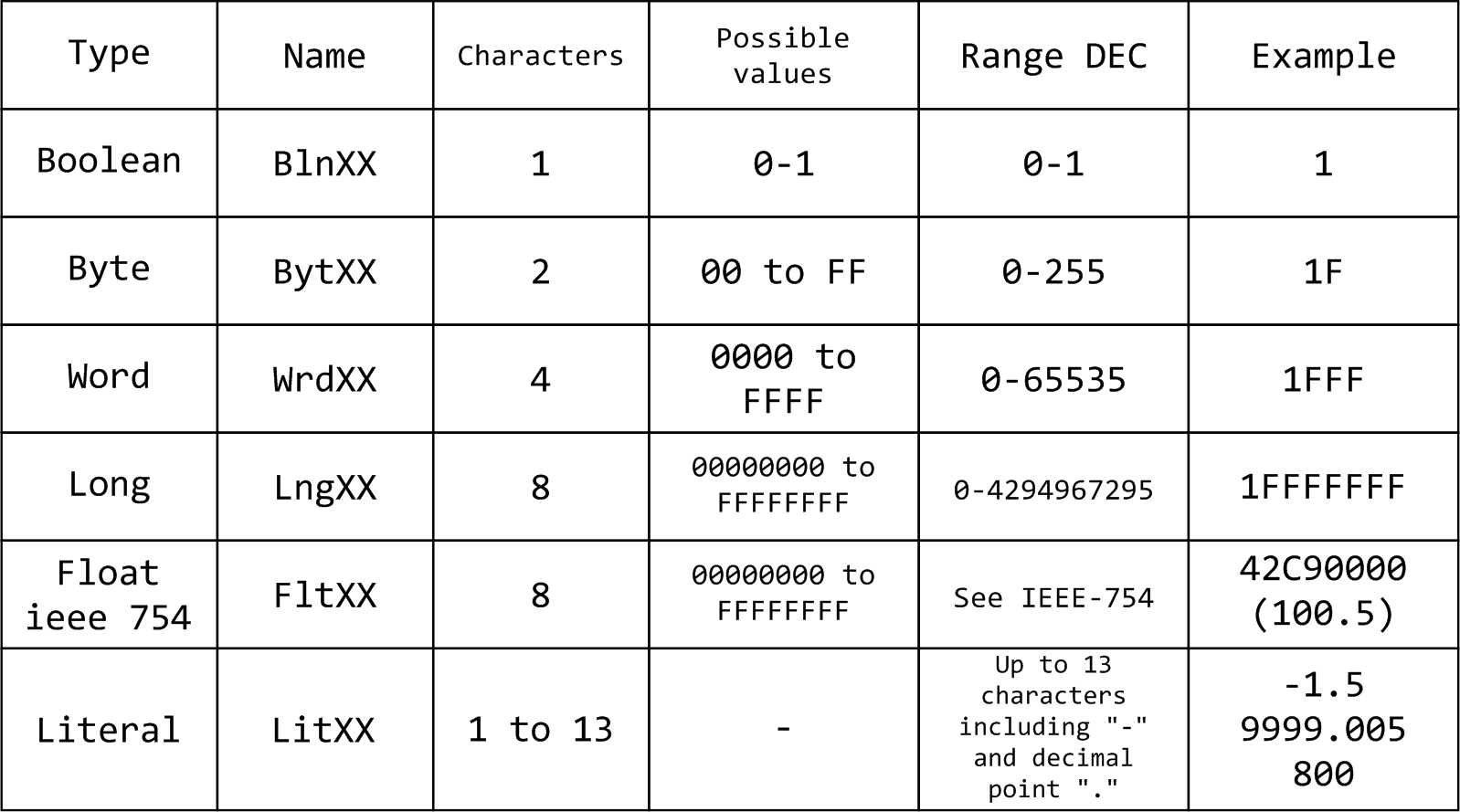
Data frame examples:
&&&&E3;XXXXXX;Bln00;Bln01;Bln02;Bln03;Byt00;Wrd00;Lng00;Flt00;Lit00;~
&FRAME1*XXXX*Lit00*Lit01*Lit02*~
For the specific case of our Project with ESP-01 and DHT-11, we will use one of the pre-defined frames called E0:
&&&&E0;XXXXXX;Lit00;Lit01;Lit02;Bln00;Bln01;~
We will assign:
; Separator character.
&&&&E0 Header that identifies the type of.
XXXXXX It is a six-character field that will occupy the sender_id.
Lit00 Relative humidity data.
Lit01 Temperature data in Celsius degrees.
Lit02 It is data. In a near future it could be used for battery level.
Bln00 It is data. In a near future it could be used for the state of relay 0.
Bln01 It is data. In a near future it could be used for the state of relay 1.
The actual frame sent by the Sender unit could be:
&&&&E0;A00001;55.1;20.3;0.0;0;0;~
Ejemplo de tramas de datos:
&&&&E3;XXXXXX;Bln00;Bln01;Bln02;Bln03;Byt00;Wrd00;Lng00;Flt00;Lit00;~
&FRAME1*XXXX*Lit00*Lit01*Lit02*~
Para el caso concreto de nuestro proyecto con Esp-01 y DHT-11 utilizaremos una de las tramas pre-definidas llamada E0:
&&&&E0;XXXXXX;Lit00;Lit01;Lit02;Bln00;Bln01;~
Asignaremos:
; Es el caracter separador.
&&&&E0 Es la cabecera que identifica el tipo de trama.
XXXXXX Es un campo de seis caracteres que ocupará el sender_id.
Lit00 Es dato, humedad relativa.
Lit01 Es dato, temperatura en grados centígrados.
Lit02 Es dato. En un futuro podría ser nivel de batería.
Bln00 Es dato. En un futuro podría representar el estado de un relé 0.
Bln01 Es dato. En un futuro podría representar el estado de un relé 1.
La trama real que envía el equipo Sender podría ser:
&&&&E0;A00001;55.1;20.3;0.0;0;0;~
New Fusdata Project
Nuevo proyecto de Fusdata
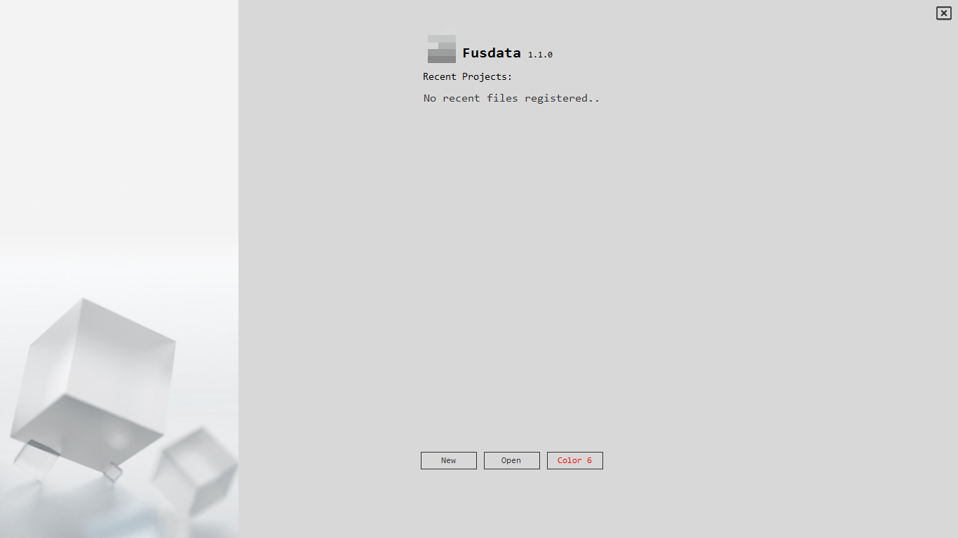
Once Fusdata is installed, to view the data from our ESP-01 we must create a new Project. Start Fusdata, click on “New” to start a new Project:
Una vez instalado Fusdata, para visualizar los datos provenientes de nuestro Esp-01 deberemos crear un nuevo proyecto. Inicia Fusdata Haz click en “New” para iniciar un nuevo proyecto:
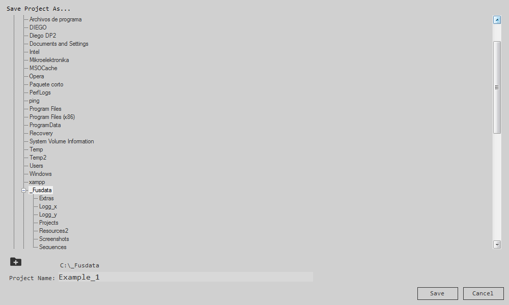
Then right-click to open the Project menú and select “Save as” to sabe the Project under a different name:
Luego haz click con el botón derecho del mouse para abrir el menú de proyecto y selecciona “Save As” para guardar el proyecto con un nombre diferente:
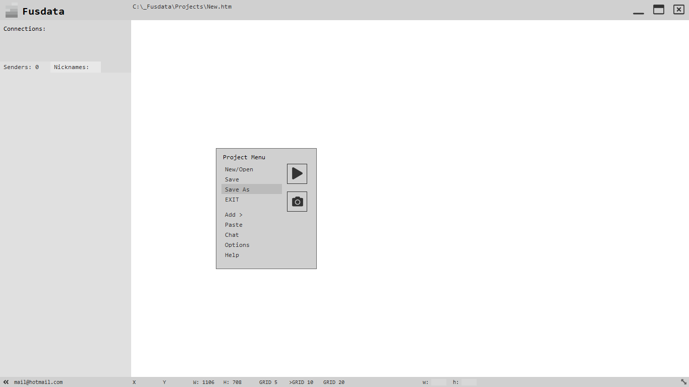
Choose a location and sabe the Project, I recommend that you sabe your Project as: C:\_Fusdata\Projects.
Elige una ubicación y guarda el proyecto, yo recomiendo que guardes tus proyectos en C:\_Fusdata\Projects.
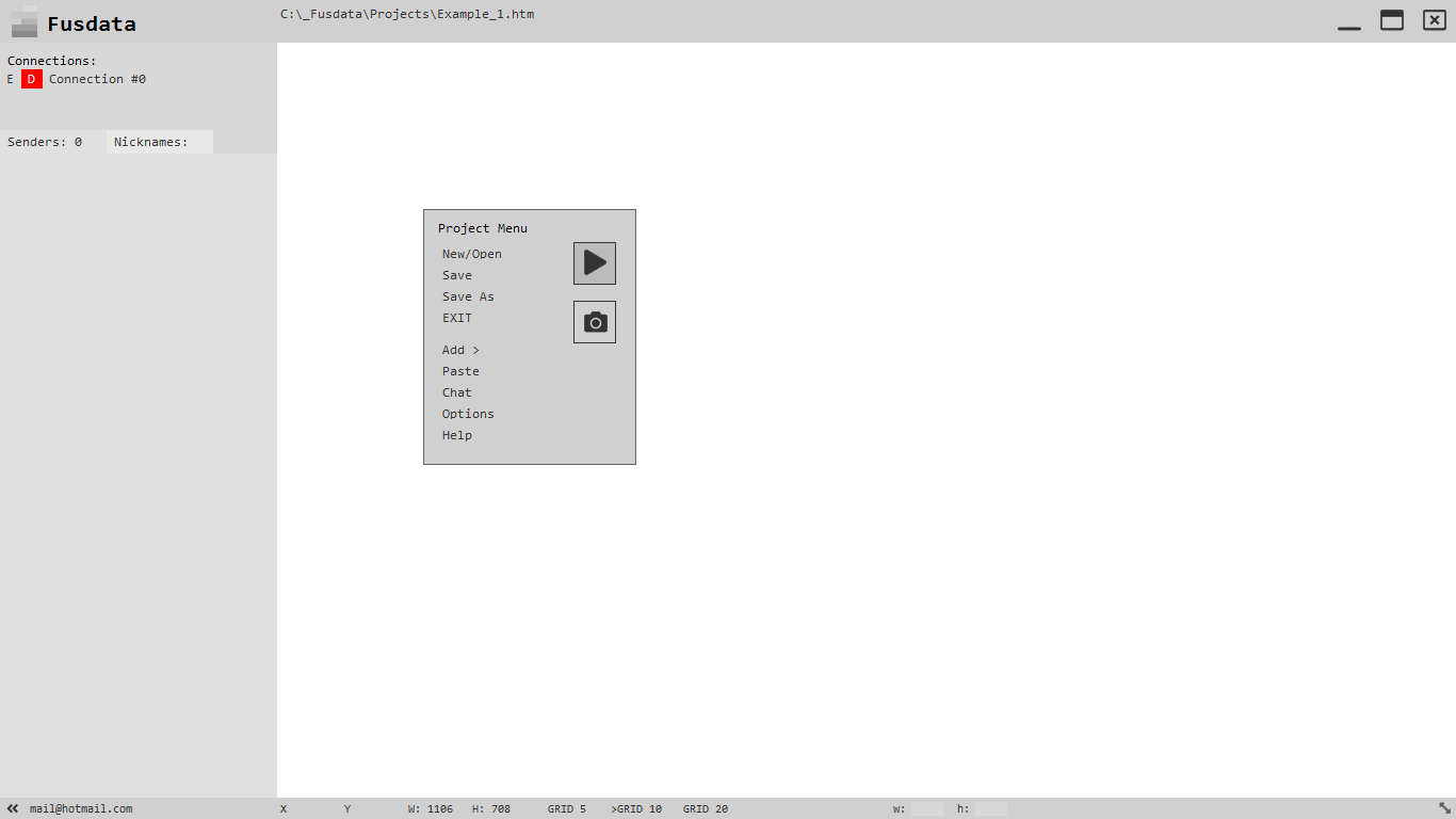
On the main screen we are going to add a new connection to a Broker MQTT. To do this, click the right mouse button and select “Add >” and then “Connection”:
Nuevamente en la pantalla principal vamos a agregar una nueva conexión con un Broker MQTT. Para ello haz click con el botón derecho del mouse y selecciona “Add >” y luego “Connection”:
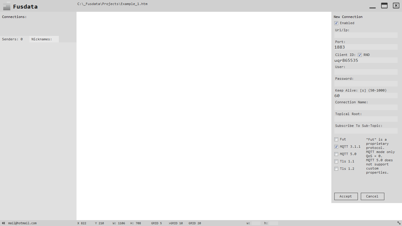
You will see that a tab appears to the right that allows you to edit the properties of the new connection with the Broker. For the purpose of continuing with the example, the parameters will be:
Y verás como aparece una solapa a la derecha que permite editar las propiedades de la nueva conexión con el Broker. A los efectos de proseguir con el ejemplo los parámetros quedarán:
Observations:
- The connection parameters are obvously the same that we have used in the firmware of our Esp-01
- The “Client ID” is generated randomly and automatically.
- The connection credentials with the Broker are not required for this example.
- The “Keep Alive” is set to 60 seconds, taking into account that the firmware recorded in the Esp-01 determined that the data is sent automatically every 12 seconds.
- The “Connection Name” parameter is optional and it is filled automatically if it is left empy.
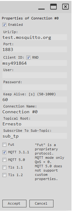
Once you have pressed accept, we will be back to the main screen with the novelty that our connection with the name “Connection #0”, appears on the left tab.
Observaciones:
- Obviamente los parámetros de conexión son los mismos que hemos puesto en el firmware de nuestro Esp-01.
- El “Client ID” se genera de manera aleatoria y automática.
- No hacen falta para este ejemplo las credenciales de conexión con el Broker.
- El “Keep Alive” queda configurado en 60 segundos teniendo en cuenta que el firmware grabado en el Esp-01 determina que los datos sean enviados automáticamente cada alrededor de 12 segundos.
- El parámetro “Connection Name” es opcional, se completa automáticamente si se deja vacío.
Una vez que hayas presionado aceptar, estaremos nuevamente en la pantalla principal, con la novedad de que ahora en la solapa de la izquierda aparece nuestra conexión con el nombre “Connection #0”.
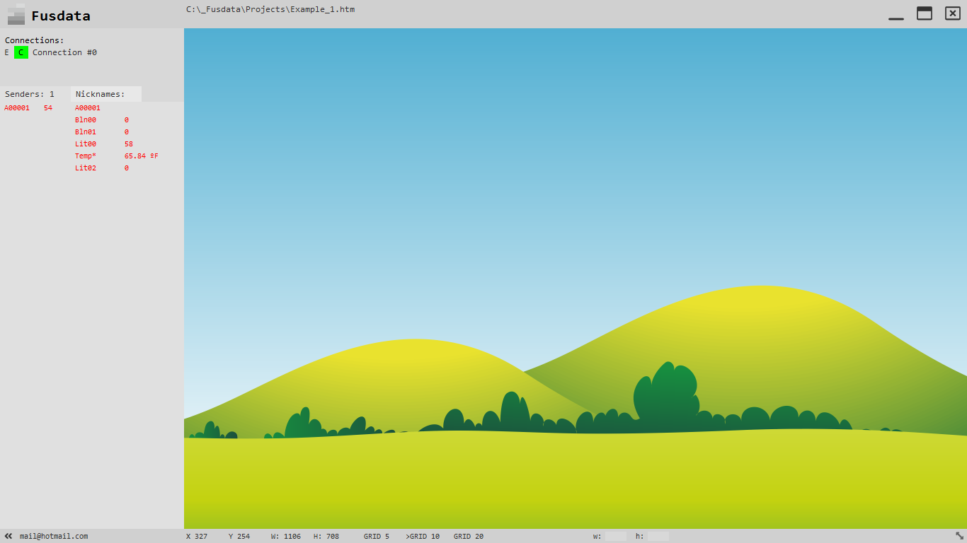
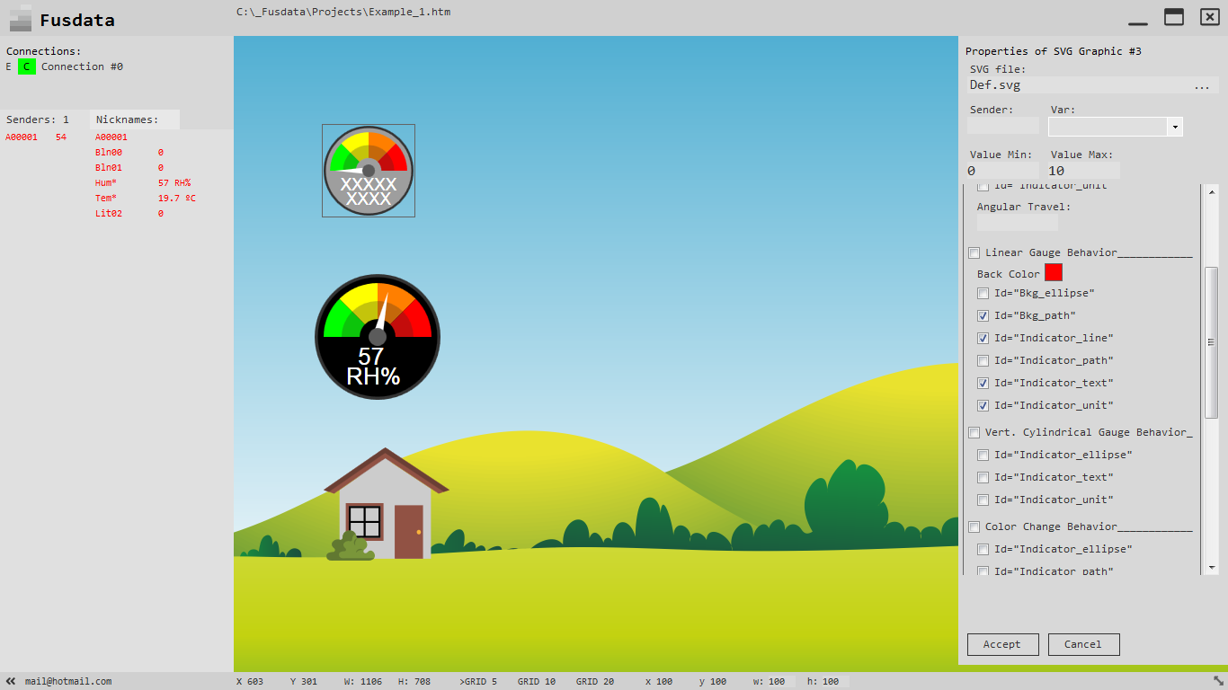
You can now click on the “Play” button in the Project menú so that the data begins to arrive form your Esp-01.You can see them by doing CTRL+2 to show and hide the data entry window.
You can also see that the status indicator has changed form red “D” to Green “C” signalling a successful connection with the Broker.
Ya puedes hacer click en el botón “Play” del menú de proyecto para que comiencen a llegar los datos desde tu Esp-01. Puedes verlos haciendo CTRL+2 para mostrar y ocultar la ventana de datos de entrada.
También puedes ver como el indicador de estado ha pasado de rojo “D” a verde “C” indicando una conexión exitosa con el Broker.
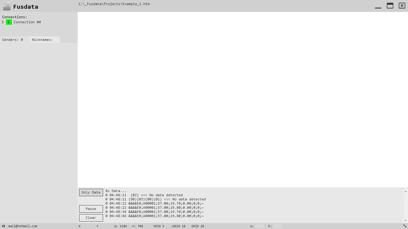
But the data as it is coming from our ESP-01 cannot be decoded until we specify the format of the data frame in Fusdata. What we should do then is to configure a new data rule in our Project menu “Add >” and then “Entry Parse Rule”. The “Data Rules Builder” will appear:
Pero los datos tal como están llegando provenientes desde nuestro Esp-01 no pueden ser decodificados hasta que especifiquemos en Fusdata el formato de la trama de datos.
Lo que debemos hacer entonces es configurar en nuestro proyecto una nueva regla de datos haciendo en el menú de proyecto “Add >” y luego “Entry Parse Rule”. Aparecerá lo que se denomina “El constructor de reglas de datos”:
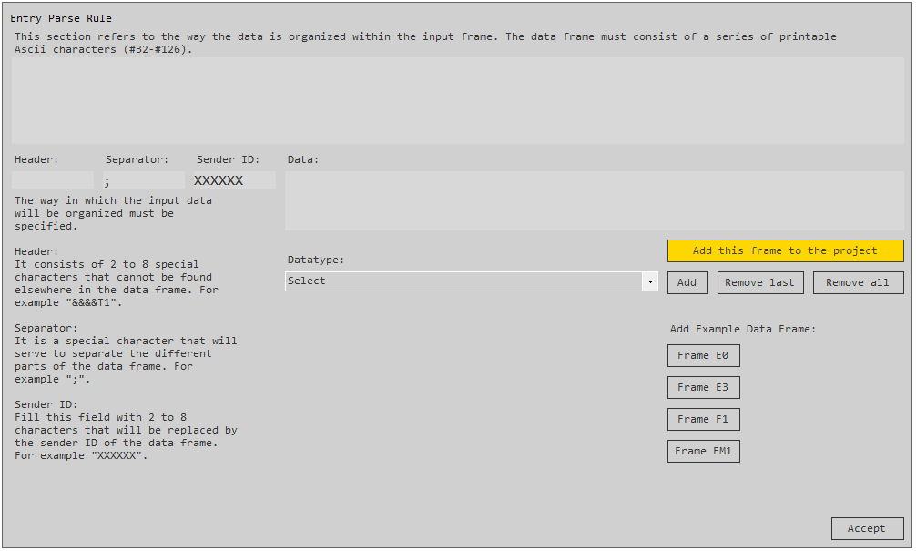
With this constructor, all the necessary types of data frames can be added to our Project. You must always specify the header, the separator carácter and the one by one the variables according to the type that we consider useful for a given Project.
Once the frame is built, we must press the yellow button “Add this frame to the Project”so that the new frame is effectively recognised by Fusdata.
Remember that our examplewith Esp-01 and DHT-11 uses a frame as:
&&&&E0;XXXXXX;Lit00;Lit01;Lit02;Bln00;Bln01;~
So,working on the data rules constructor, you will have:
Con este constructor pueden agregarse a nuestro proyecto todas los tipos de trama de datos que sean necesarias. Siempre debe especificarse la cabecera, el caracter separador y a continuación una a una las variables según el tipo que consideremos útil para un proyecto determinado.
Una vez construida la trama deberemos presionar el botón amarillo “Add this frame to the project” para que efectivamente la nueva trama sea reconocida por Fusdata.
Recordemos que nuestro ejemplo con Esp-01 y DHT-11 emplea una trama donde:
&&&&E0;XXXXXX;Lit00;Lit01;Lit02;Bln00;Bln01;~
Entonces, trabajando sobre el constructor de reglas de datos, quedará:
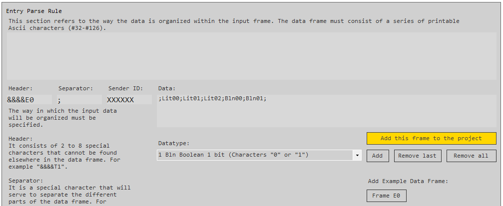
And as we said, we should press the yellow button to add the new plot to our project:
Y como dijimos deberemos presionar el botón amarillo para agregar la nueva trama al proyecto:
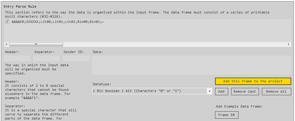
I shall clariry that that for this type of frame that we call “Frame E0”, there is an example frame button that automatically builds the entire frame.
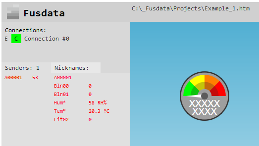
At this point our Project already recieves the data form our Esp-01 and the Fusdata can decode the frame and the values are presented in the tab, to the left:
Aclaro que en particular para este tipo de trama a la que denominamos “E0” hay un botón de tramas de ejemplo que construye automáticamente toda la trama “Frame E0”.
A estas alturas nuestro proyecto ya recibe los datos desde nuestro Esp-01 y Fusdata puede decodificar la trama y los valores se presentan en la solapa de la izquierda:

You can see the names of the variables and their raw values as they are sent by Sender A00001. Being:
Relative humidity: 55 %
Temperature: 20.1 ºC
The unit with which each unit is presented, is determined by convention and was defined at the time of developing the firmware that is hosted in our ESP-01. In any case, it is always posible to transform the data as we will see later.
Also note that the order in which the variables appear is not necessarily the order in which they appear in the data frame.
IMPORTANT NOTE: Remember that after modifying any characteristic of a Project you must save the changes from the Project menú with “Save” or by pressing CTRL+S.
Pueden verse los nombres de las variables y sus valores crudos tal cual son enviados por el Sender A00001. Siendo:
Humedad relativa: 55 %
Temperatura: 20.1 ºC
La unidad con la que se presenta cada magnitud está determinada por convención y se definió al momento de desarrollar el firmware que se aloja en nuestro Esp-01. De todas maneras siempre es posible transformar los datos como veremos más adelante.
Observa también que el orden en el que aparecen las variables no es necesariamente el que tienen en la trama de datos.
NOTA IMPORTANTE: Recuerda que luego de modificar cualquier característica de un proyecto debes grabar los cambios desde el menú de proyecto con “Save” o haciendo CTRL+S.
How to transform the received data
Como transformar los datos recibidos
The data sent by the sender has the format that has been determined at the momento of making the firmware, and the units in which they are expressed can be implicit.Sometimes even raw data is transmitted just as it is in the internal registers of the microprocessor.
For example, we can mention the case of a pressure sensor wityh a 0-5V output that is connected to an analog input of a Sender device.The data obtained may be sent as it is contained in the internal register of the analog-digital converter.
Then in Fusdata and each particular Project we can transform the raw data through a mathematical function to a value that reflects the true physical parameter that is being measured.
Continuing with the example that we have been dealing with in this entry, suppose we want to obsere the temparature data in Fahrenheit degrees, as we know the formula to transform the Celsiuos degrees to Fahrenheit degrees:
y = (1.8*x) + 32
Where “y” represents the temperature value in ºF and “x” the value in ºC.
Los datos enviados por el Sender tienen el formato que se ha determinado al momento de realizar el firmware, y las unidades en que se expresan pueden estar implícitas. A veces incluso los datos son transmitidos crudos, tal cual se encuentran en los registros internos del micro procesador.
Por ejemplo podemos mencionar el caso de un sensor de presión con salida 0-5V que se conecta a una entrada analógica de un dispositivo Sender. Puede ser que el dato obtenido sea enviado tal cual está contenido en el registro interno del conversor analógico-digital.
Luego en Fusdata y en cada proyecto en particular podemos transformar el dato crudo mediante una función matemática a un valor que refleje el verdadero parámetro físico que se está midiendo.
Siguiendo con el ejemplo que venimos tratando en esta entrada, supongamos que deseamos observar los datos de temperatura en grados Fahrenheit, como sabemos la fórmula para transformar grados Centígrados a grados Fahrenheit es:
y = (1.8*x) + 32
Donde “y” representa el valor de temperatura en ºF y “x” el valor en ºC.
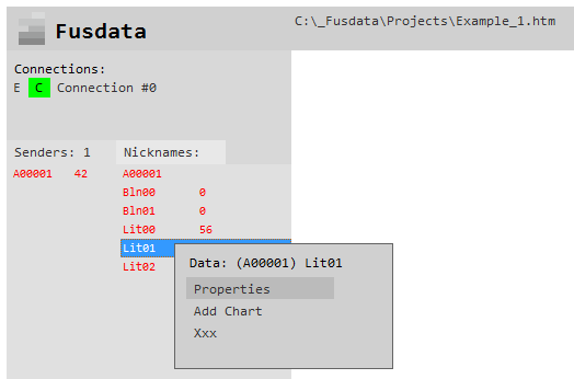
Then, to include this transformation in a Fusdata Project we must click with the right mouse button on the value of the variable that we want to transform in the data list within thhe data tab and choose “properties”:
Luego para incluir esta transformación en un proyecto de Fusdata debemos hacer click con el botón derecho del mouse sobre el valor de la variable que queremos transformar en la lista de datos en la solapa de datos y elegir “Properties”:
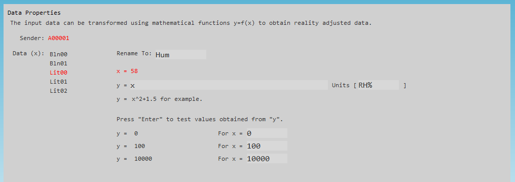
A transformation properties screen will automatically appear for the variable “Lit01”:
Automáticamente aparecerá una pantalla de propiedades de transformación para la variable “Lit01”:
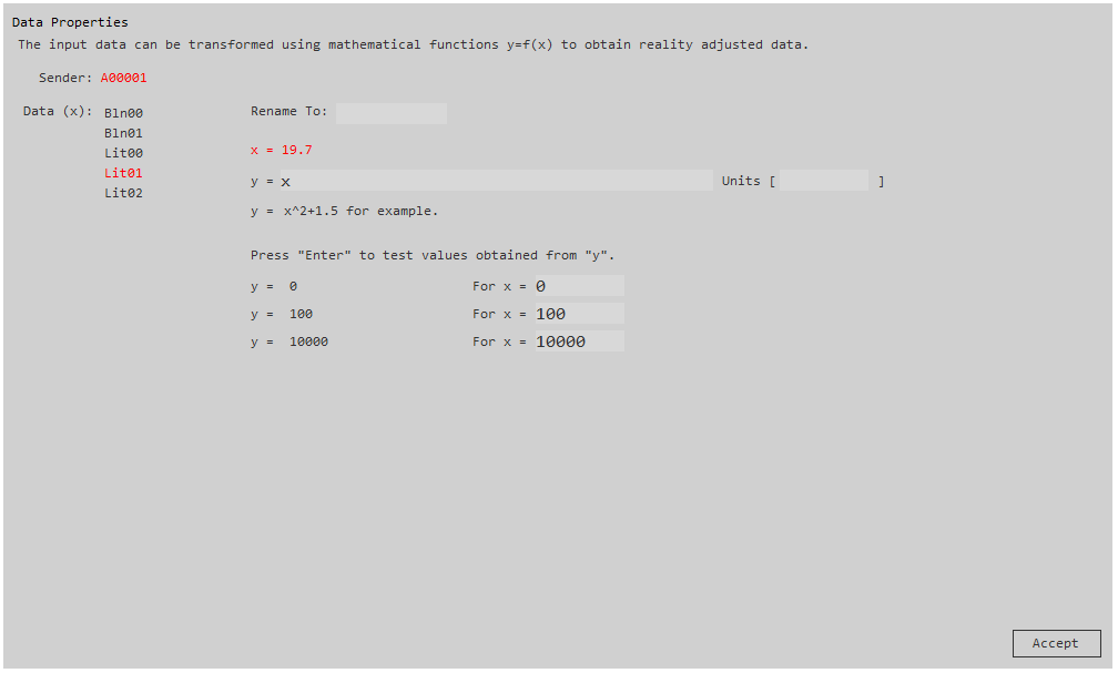
Here we can enter a transformation formula for the value of Lit01 to obtain the temperature measurement in ºF:
Aquí podremos ingresar una fórmula de transformación para el valor de Lit01 para obtener la medida de temperatura en ºF:
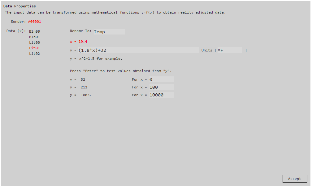
We also take the opportunity to specify that the uit of measurement is “ºF” and that in the data list we will see the variable Lit01 as “Temp” which will give us a clearer idea of the magnitude measured at naked eye.
Then, with the arrival of new data from the Sender at issue, it will be posible to observe the changes:
Y aprovechamos también para especificar que la unidad de medida es “ºF” y que en la lista de datos veremos a la variable Lit01 como “Temp” lo que nos dará una idea más clara de la magnitud medida a simple vista.
Luego, con el arribo de nuevos datos provenientes del Sender en cuestión se podrán observar los cambios:
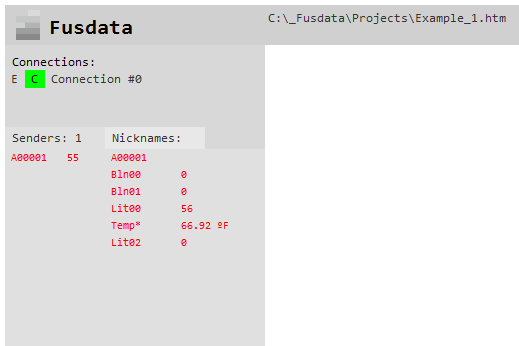
Notice that now the variable Lit01 appears as “Temp” with a value in ºFNote also that an asterisk“*”appears, which indicates a variable has been transformed.
It should be mentioned now that this modificarion is only valid for the Lit01 variable of the Sender A00001 and in this particular Project, if we have many Senders devices to which we also perform this transformation on the Lit01 variable of each one, the process could be quite tedious.
For thios reason, perhaps the best thing would be to make a good approach in the firmware design stage, to minimize the process of variable transformationsOn the other hand, this possibility of inserting variable transformations gives the sistema great flexibility. Le us imagine for example, that the Sender device design can send different types of measurements in the same variable.In other words, let us think that we could design a single model of Sender devices whose analog inputs could be connected to different types of analog sensors and thus, for example, the Lit01 variable in one device can represent a pressure and in another device it coul represent a liquid level.
Observemos que ahora la variable Lit01 aparece como “Temp” con un valor en ºF. Notemos también que aparece un asterisco “*”, esto indica que esta variable ha sido transformada.
Hay que mencionar ahora que esta modificación solo es válida para la variable Lit01 del Sender A00001 y en este proyecto en particular, si tuviéramos muchos equipos Sender a los que realizar también dicha transformación en la variable Lit01 de cada uno, el proceso podría ser bastante tedioso. Por ello quizás lo mejor sería hacer un buen planteo en la etapa de diseño del firmware para minimizar el proceso de transformaciones de variables. Por contrapartida esta posibilidad de insertar trasformaciones de variables otorga gran flexibilidad al sistema, imaginemos por ejemplo que un mismo diseño de dispositivo Sender pueden enviar diferentes tipos de medidas en la misma variable. O sea pensemos que podríamos diseñar un único modelo de dispositivos Sender cuyas entradas analógicas pudieran estar conectados a diferentes tipos de sensores analógicos y así por ejemplo la variable Lit01 en un dispositivo puede representar una presión y en otro dispositivo puede ser un nivel de líquido.
Creation of historical records
Creación de registros históricos
By default, Fusdata does not record data when we créate a new Project.To enable this function, you must select “Options” from the Project menu and enable the corresponding box in the options menu.
Por default Fusdata no realiza el registro de datos cuando creamos un nuevo proyecto. Para habilitar esta función se debe selecciones “Options” del menú de proyecto y habilitar la casilla correspondiente del menú de opciones.
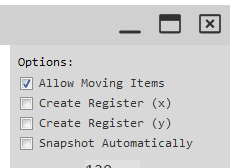
As you can see there are two boxes:
- “Create Register (x)” which enables the creation of the record for the variables as they arrive from the Sender without transfortmation.
- “Create Register (y)” which enables the creation of the record but replaces a given variable “x” if there is a transformation “y” for said variable.
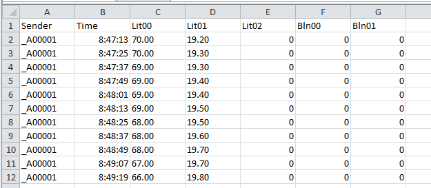
The logs are simple text files in .CVS format that can be viewed with any text editor or spreadsheet. Each file created as a record, corresponds to a full day of data frorm the time 00:00:00 and will have the name: data yyyy-mm-dd.csv.
The “X” registers will be logged inside the files structure:
C:\_Fusdata\Logg_x\yyyy\_device_id
Como puede verse existen dos casillas:
- “Create Register (x)” que habilita la creación del registro para las variables tal y como llegan del Sender sin transformación.
- “Create Register (y)” que habilita la creación del registro pero remplaza una variable “x” determinada si es que existiese una transformación “y” para dicha variable.
Los registros son simples archivos de texto en formato .CSV que pueden verse con cualquier editor de texto o planilla de cálculo. Cada archivo creado como registro corresponde a un día completo de datos recibidos desde la hora 00:00:00 y tendrá el nombre yyyy-mm-dd.csv.
Los registros “x” se alojan dentro de la estructura de carpetas:
C:\_Fusdata\Logg_x\yyyy\_device_id
The “y” registers will be created inside the structure:
C:\_Fusdata\Logg_y\yyyy\_device_id
Y los registros “y” se crean dentro de la estructura:
C:\_Fusdata\Logg_y\yyyy\_device_id
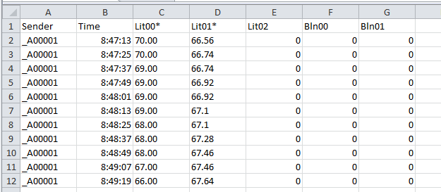
As can be seen, both registers only differ in the value that Lit01 takes, which can have an original value in ºC for the “x” register as it was sent by the Sendero r a value transformed to ºF for “y” register.
These register files are also used by the charts that can be included in a Fusdata Project as we will see later.
Como puede verse ambos registros solo difieren en el valor que toma Lit01 que puede tener un valor original en ºC para el registro “x” según fue enviado por el Sender o un valor transformado a ºF para el registro “y”.
Estos archivos de registro también son utilizados por los gráficos Charts que pueden incluirse en un proyecto de Fusdata como veremos más adelante.
Record creation strategy
Estrategia de creación de registros
If we think about it, we see that each Fusdata Project can create records, and since we can have projects running simultaneously on our computer, the parameters received for each project would record so multiple recods of the same value will be created.
For this reason, it is necessary to select the particular Project that will be enabled for the creation of historical records. Sometimes even a Fusdata project can have the only function of creating said records.
Si lo pensamos bien, vemos que cada proyecto de Fusdata puede crear registros, y como podemos tener proyectos corriendo en simultáneo en nuestra computadora, puede que los parámetros recibidos por cada proyecto se graben por lo que se crearán múltiples registros del mismo valor. Esta situación ocasiona sobrecarga del sistema y no es conveniente.
Por ello hay que seleccionar el proyecto particular que será el que sea habilitado para la creación de los registros históricos. A veces incluso un proyecto de Fusdata puede tener como única función la creación de dichos registros.
Dashboard graphic develepment
Desarrollo gráfico del tablero de control
To provide a greater number of creative options, Fusdata is in ongoing develpment so new features are added version by version.
To begin with, let us take into account that Fusdata provides a working areain which different elements can be arranged together to form an interface that will allow interactions with bidirectionl dynamics Seder devices in real time.The idea is to créate a true board to control what we want, no matter how far away or in what part of the world it is.
And once again, returning to the practical example of relative humidity and temperatura measurement with Esp-01 and Fusdata using the MQTT protocol, I think that the most beautiful and interesting thing is just what we have to do…which is the display of the data on the screen to obtain a didactic and engaging interface on our Project.
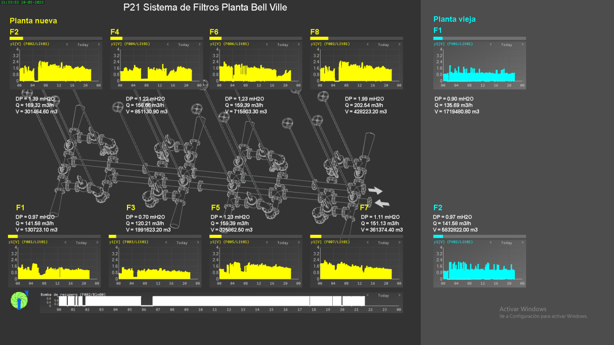
What we see below represents a sand filter room in a wáter purification plant. In it, the instantaneous flows in each filter are measured by measuring the differential pressure present in the corresponding Venturi tube. This screen is used to erify at a glance the correct operation of the ten filters and to identify the posible saturation of any of them, which will aloow to plan their cleaning and restoration to full operation.
Para dar mayor número de alternativas creativas, Fusdata se encuentra en permanente desarrollo y versión a versión se irán incorporando novedades.
Para empezar tengamos en cuenta que Fusdata proporciona un área de trabajo en la que se pueden disponer distintos elementos que juntos conformarán una interface que permitirá interactuar con los dispositivos Sender con una dinámica bidireccional en tiempo real de datos. La idea es crear un verdadero tablero para controlar eso que deseamos sin importar qué tan lejos o en qué parte del mundo se encuentre.
Y nuevamente regresando al ejemplo práctico de medición de humedad relativa y temperatura con un Esp-01 y Fusdata utilizando el protocolo MQTT creo que lo más lindo e interesante es justo lo que nos queda por hacer… que es el despliegue de los datos en la pantalla para obtener una interface didáctica y atractiva sobre nuestro proyecto.
Esto que vemos a continuación representa una sala de filtros de arena en una planta de potabilizadora de agua. En ella se miden los caudales instantáneos en cada filtro mediante la medición de la presión diferencial presente en el correspondiente tubo Venturi. Esta pantalla se utiliza para verificar a golpe de vista el correcto funcionamiento de los diez filtros e identificar la posible saturación de alguno de ellos, lo que posibilitará planificar su limpieza y restauración a pleno funcionamiento.
Background image of our project
Imágen de fondo de nuestro proyecto
In my opinión the creation the scene begins by having a background image that allow us to establish a framwork and a clear idea of what we are controlling.
To add a background to our Project we must choose “Add >” and then “Background”, a file explorer will immediately open and it will allow us to search for a previously conditioned image to use as a background .
The size of the image that we select and use as a background of the project will be decisive in the design.
En mi opinión la creación de la escena comienza por disponer de una imagen de fondo que permita establecer un marco y una idea clara sobre lo que estamos controlando.
Para agregar un fondo a nuestro proyecto debemos elegir en el menú de proyecto “Add >” y luego “Background”, inmediatamente se abrirá un explorador de archivos que permitirá buscar una imagen previamente acondicionada para utilizar como fondo.
El tamaño de la imagen que utilicemos como fondo de proyecto será determinante en el diseño.
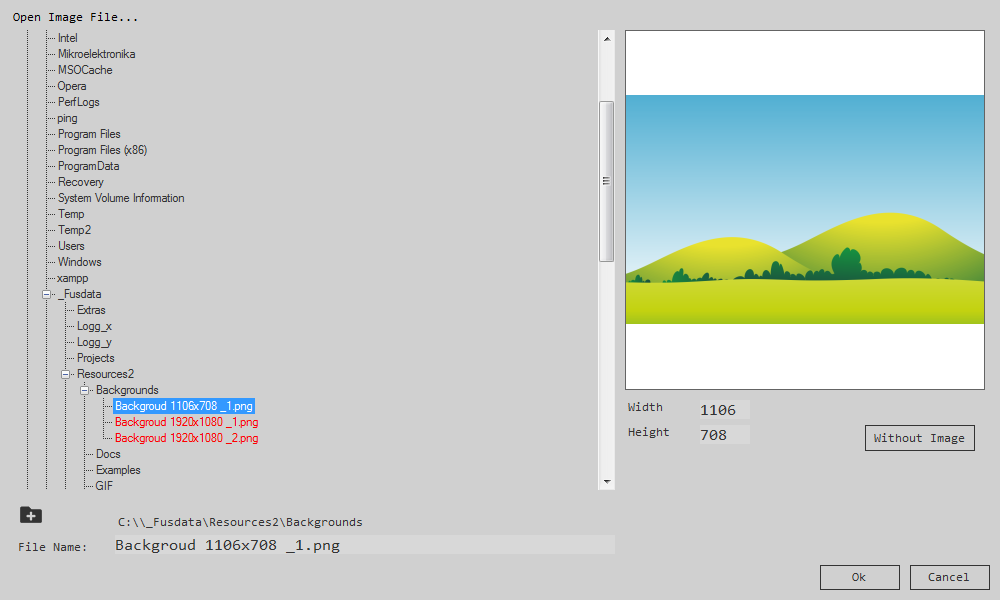
The background for this Project can be found in:
C:\_Fusdata\Resources2\Backgrounds\Backgroud 1106×708 _1.png
We select the file and press OK so that the Project can be displayed as follows:
El fondo para este ejemplo se encuentra en:
C:\_Fusdata\Resources2\Backgrounds\Backgroud 1106×708 _1.png
Seleccionamos el archivo y presionamos Ok para que el proyecto ahora se muestre de la siguiente manera:
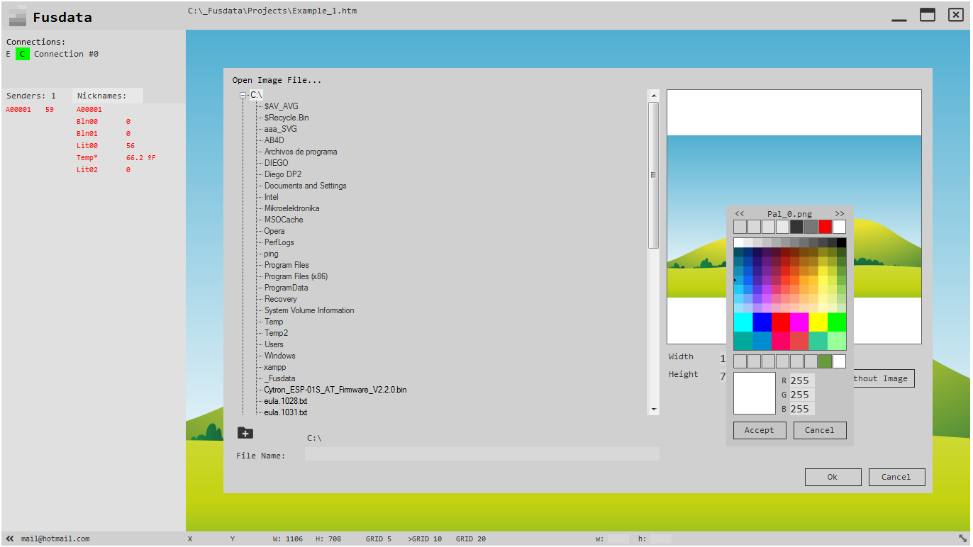
At any time you can modify the backgropund ore ven remove it with the “Whitouth Image” button to only display a solid color that can be selected by clicking on the preview area:
En cualquier momento se puede modificar el fondo o incluso removerlo con el botón “Whitouth Image” para solo visualizar un color sólido que se puede seleccionar haciendo clic sobre el área de pre-visualización:
Add an SVG graphic
Agregar un gráfico SVG
An SVG graphic has the particularity of not losing resolution when resized, which allows the image quality to be preserved. In Fusdata you can ad done by doing “Add >” and then “SVG Graphic”.
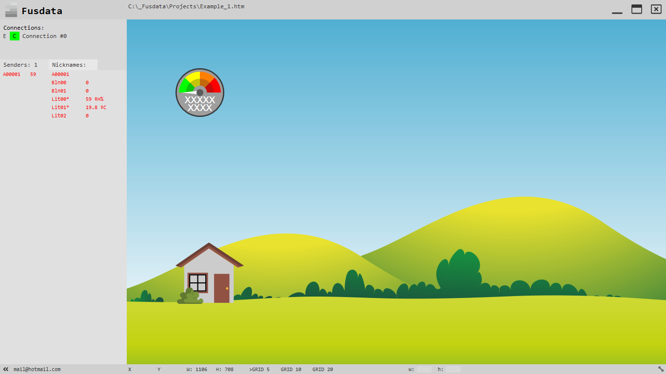
A default graphic Def.svg will automatically appear on the screen.
Then if we click the right mouse button on it, we Access the properties tab:
Un gráfico SVG tiene la particularidad de no perder resolución al cambiar de tamaño, lo que permite conservar la calidad de la imagen. En Fusdata puedes agregar uno haciendo “Add >” y luego “SVG Graphic”.
Aparecerá automáticamente un gráfico por default Def.svg en pantalla.
Luego si hacemos click con el botón derecho del mouse sobre él, accedemos a la solapa de propiedades:
In this tab you can see the name of the file at the top right and a button with three points “…” that will allow us to choose a different SVG graphic , if we press itthe file explorer will open and we can navigate and select a small house:
En dicha solapa puede observarse arriba a la derecha el nombre del archivo y un botón con tres puntos ”…” que nos permitirá elegir un gráfico SVG distinto, si lo presionamos se abrirá el explorador de archivos y podremos navegar y seleccionar una pequeña casita:
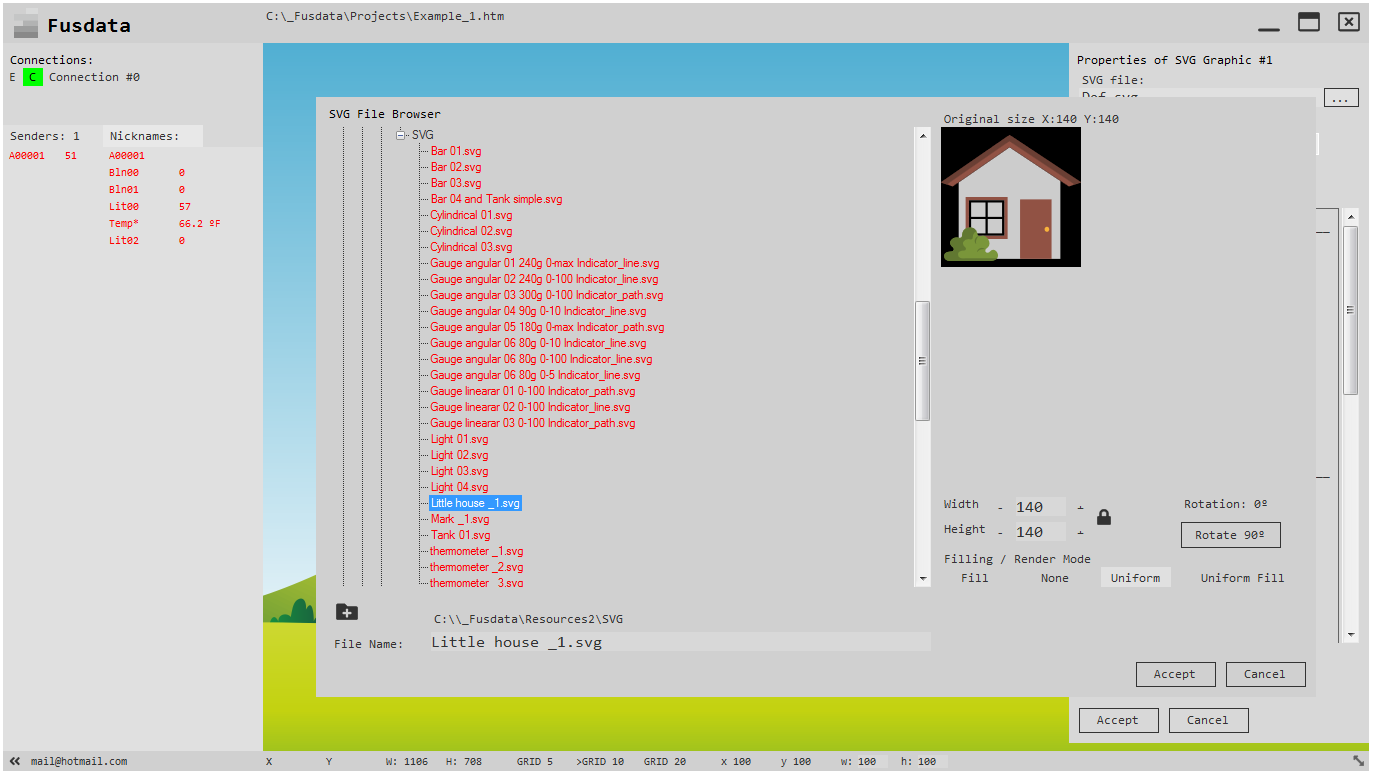
This file is located in:
C:\_Fusdata\Resources2\SVG\Little house _1.svg
Staying:
Este archivo se encuentra en:
C:\_Fusdata\Resources2\SVG\Little house _1.svg
Quedando:
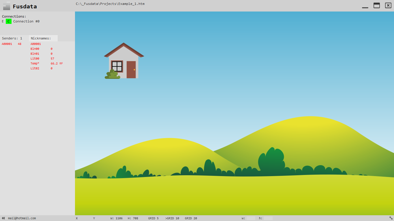
This SVG object is loose and can be dragged and dropped wherever we want:
Este objeto SVG se encuentra suelto y puede arrastrarse y colocarse donde se desee:
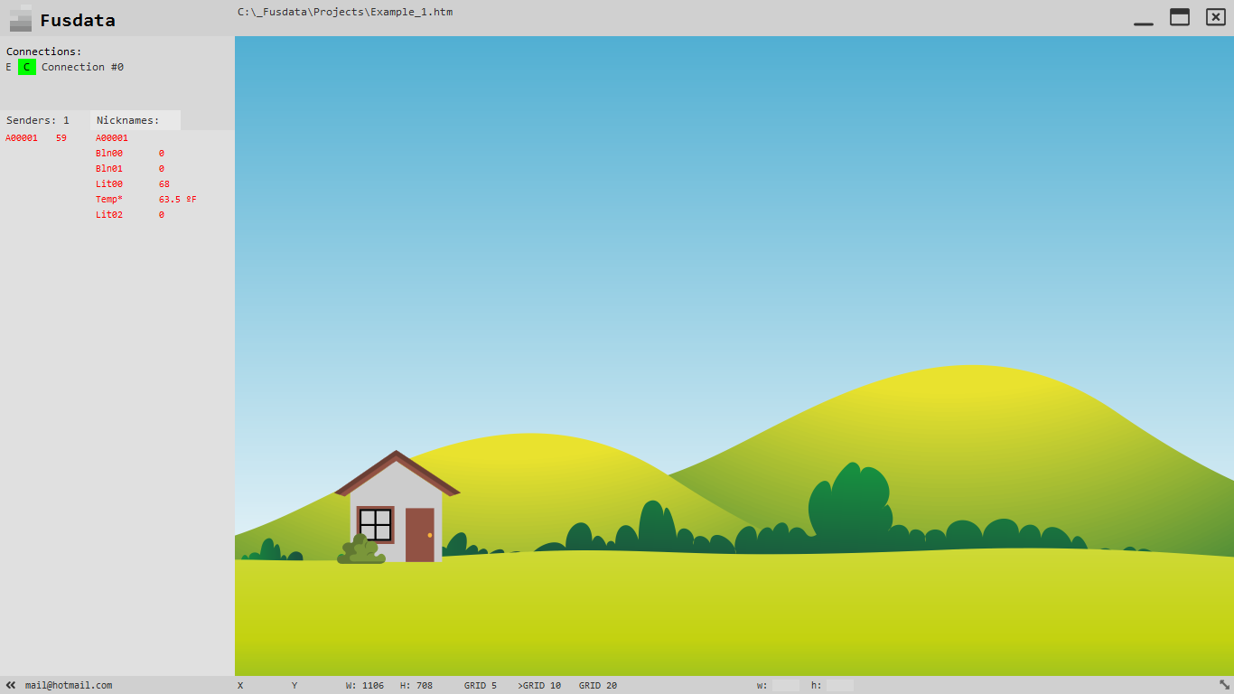
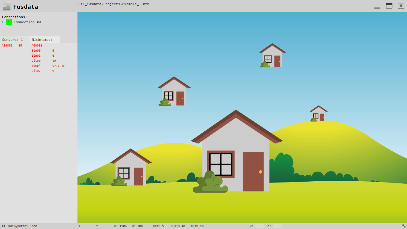
Other modifications that we can make on a SVG graphic are:
Ctrl + D To duplicate the selecte item.
Ctrl + + To proportionally increase the size of the selected item.
Ctrl + – To proportionally dicrease the size of the selected item.
Ctrl + Right To increase the size of the selected ítem only on the axis X.
Ctrl + Left To dicrease the size of the selected ítem only on the axis X.
Ctrl + Down To increase the size of the selected ítem only on the axis Y.
Ctrl + Up To dicrease the size of the selected ítem only on the axis Y.
Alt + Right To move the selecte ítem to the right.
Alt + Left To move the selecte ítem to the left.
Alt + Up To move the selecte ítem up.
Alt + Down To move the selecte ítem down.
Otras modificaciones que podemos hacer sobre el gráfico SVG son:
Ctrl + D Para duplicar el elemento seleccionado.
Ctrl + + Para aumentar proporcionalmente el tamaño del elemento seleccionado.
Ctrl + – Para disminuir proporcionalmente el tamaño del elemento seleccionado.
Ctrl + Right Para aumentar el tamaño del elemento seleccionado solo en el eje X.
Ctrl + Left Para disminuir el tamaño del elemento seleccionado solo en el eje X.
Ctrl + Down Para aumentar el tamaño del elemento seleccionado solo en el eje Y.
Ctrl + Up Para disminuir el tamaño del elemento seleccionado solo en el eje Y.
Alt + Right Para mover el elemento seleccionado hacia la derecha.
Alt + Left Para mover el elemento seleccionado hacia la izquierda.
Alt + Up Para mover el elemento seleccionado hacia arriba.
Alt + Down Para mover el elemento seleccionado hacia abajo.
Add an SVG dial to display relative humidity
Agregar un cuadrante SVG para mostrar la humedad relativa
We will add another SVG graphic to work as a virtual instrument. We should understand that an .svg file is a simple text file in which there is a code that Fusdata interprets and executes to créate the graphic on the screen .This logic characterisctic of the SVG format that allows the drawingto not loose quality regardless of its size.
Fusdata is capable of inserting an SVG file into the Project and manipulating its constituent elements so that this drawing reflects the value of a variable.For example the needle of a clock-type dial can be rotated so that it indicates certain value
You should specify at the time of Project creation which will be the elements of the SVG file to be modified by Fusdata in order to obtain a transformation of the drawing.
Vamos a agregar ahora otro gráfico SVG para que funcione como un instrumento virtual. Debemos entender que un archivo .svg es un simple archivo de texto en el que se encuentra un código que Fusdata interpreta y ejecuta para crear el gráfico en pantalla, esta lógica característica del formato SVG es lo que permite que el dibujo no pierda calidad independientemente de su tamaño.
Fusdata es capaz de insertar en el proyecto un archivo SVG y manipular sus elementos constitutivos para que este dibujo refleje el valor de una variable. Por ejemplo se puede hacer girar la aguja de un cuadrante tipo reloj para que indique un valor determinado.
Tú debes especificar al momento de la creación del proyecto cuáles serán los elementos del archivo SVG a modificar por Fusdata para obtener así una transformación del dibujo. Dependerán esas especificaciones del propio archivo elegido y del efecto visual deseado.
The idea is to make a clok-type dial that indicates the level of relative humidity. To do this, we fisrt modify the properties of the Lit00 and Lit01 variables so that they incorpórate the corresponding units. It is not a transformation itself but you can proceed in this way:
La idea es hacer un cuadrante tipo reloj que nos indique el nivel de humedad relativa. Para ello primero modificamos las propiedades de las variables Lit00 y Lit01 para que incorporen las unidades correspondientes. No es una transformación propiamente dicha pero se procede de la misma manera:

In this way we achieve that the list of input variables:
Así logramos que la lista de variables de entrada quede de la siguiente forma:
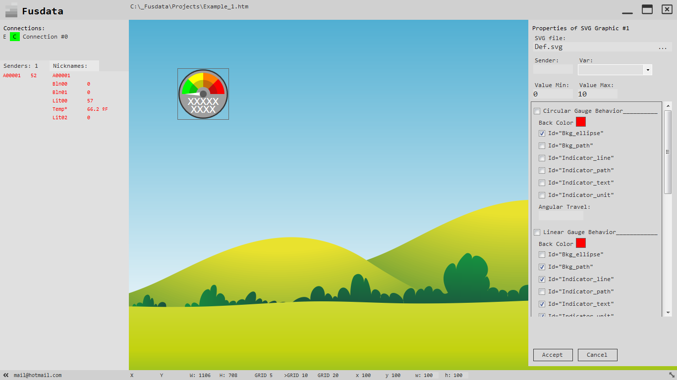
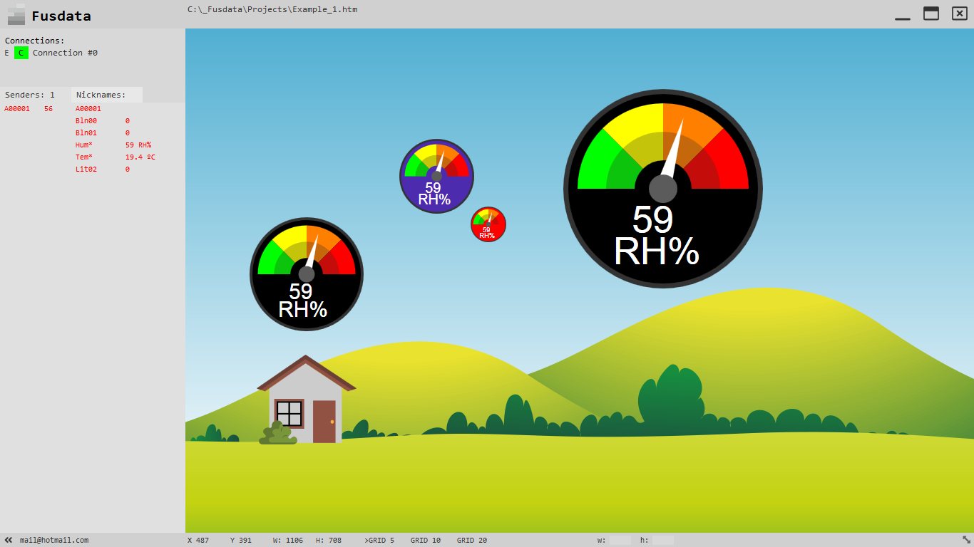
In the same way as before, we Access the porperties of the SVG graphicto be able to to model its behaivour to reflect the humidity valu for Sender A00001:
De la misma manera que antes, accedemos a las propiedades del gráfico SVG para poder modelar su comportamiento para que refleje el valor de humedad relativa para el Sender A00001:
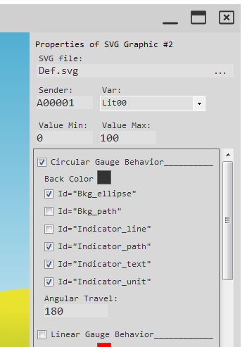
You can see in the figure all the properties to take into account:
SVG file: Def.svg SVG file.
Sender: A00001 It is the sender_id of the device that sends the data.
Var: Lit00 It is the “relative humidity” variable.
Value Min: 0 Hypothetical value with which the needle points to the minimum.
Value Max: 100 Hypothetical value with which the needle points to full scale.
Having selected this file as an SVG graphic, it is defined that we are talking about a circulasr dial or “Circular Gaugetjhat is, just by looking at the shape of the graphic we realice the type of behavoir it will have.That is why we check the “Circular Gauge Behavior” box.
The SVG file has internal elements with names, in fact it is a tag file where the different elements that compose it also have well-defined properties. You can also learn more about SVG graphics in:
www.w3.org/Graphics/SVG/
www.w3schools.com/graphics/svg_intro.asp
In a future entry I will explain in more detail how SVG files work in Fusdata and the features it must have so that you can make them yourself with the help of very good free software called Inkscape.
We may well suspect that there is a circular or elliptical element called “Bkg_ellipse” taht makes uo the background of this SVG file3, and so we check the “Id=Bkg_ellipse”box. This constitutive element of the SVG file will be the one that becomes the color chosen in the option “Back color”.
With any text editor we can open the file and check that said element is present:
<circle fill=”#9e9e9e” cx=”100″ cy=”100″ id=”Bkg_ellipse” r=”95″ />
Se pueden ver en la figura todas las propiedades a tener en cuenta:
SVG file: Def.svg Archivo SVG.
Sender: A00001 Es el sender_id del dispositivo que envía el dato.
Var: Lit00 Que es la variable “Humedad relativa”.
Value Min: 0 Hipotético valor con el que la aguja señala el mínimo.
Value Max: 100 Hipotético valor con el que la aguja señala fondo de escala.
Al haber seleccionado este archivo como gráfico SVG queda definido que estamos hablando de un cuadrante circular o “Circular Gauge”, o sea, con solo observar la forma del gráfico nos damos cuenta del tipo de comportamiento que tendrá. Por ello marcamos la casilla “Circular Gauge Behavior”.
El archivo SVG tiene elementos internos con nombres, de hecho es un archivo de etiquetas donde los diferentes elementos que lo componen tienen también propiedades bien definidas. Se puede aprender más sobre gráficos SVG en:
www.w3.org/Graphics/SVG/
www.w3schools.com/graphics/svg_intro.asp
En una futura entrada voy a explicar en mayor detalle el funcionamiento de los archivos SVG en Fusdata y las características que debe tener para que tú mismo puedas hacerlos con la ayuda de un software gratuito y muy bueno llamado Inkscape.
Podemos sospechar con muchas chances de tener razón que hay un elemento circular o elíptico llamado “Bkg_ellipse” que compone el fondo de este archivo SVG, y entonces marcamos la casilla “Id=Bkg_ellipse”. Este elemento constitutivo del archivo SVG será el que se torne del color elegido en la opción “Back Color”.
Con cualquier editor de texto podemos abrir el archivo y comprobar que dicho elemento se encuentra presente:
<circle fill=”#9e9e9e” cx=”100″ cy=”100″ id=”Bkg_ellipse” r=”95″ />
Depending on the shape of the figure that determines the background of the chosen SVG graphic , it may happen that the box to choose is “Bkg_path” as it would be in the case of this other file:
Dependiendo de la forma de la figura que determina el fondo del gráfico SVG elegido puede ocurrir que la casilla a elegir sea “Bkg_path” como sería en el caso de este otro archivo:
File that can be found in:
C:\_Fusdata\Resources2\SVG\Gauge angular 04 90g 0-10 Indicator_line.svg
And, as we can check using any text editor, we will find an elemant called “Id=Bkg_path”:
<path d=”M26.087 26.087v347.826h347.826V26.087z” id=”Bkg_path” fill=”#9e9e9e”…
Este archive se encuentra en:
C:\_Fusdata\Resources2\SVG\Gauge angular 04 90g 0-10 Indicator_line.svg
Y, como podemos verificar utilizando cualquier editor de texto, observamos que se encuentra un elemento denominado “Id=Bkg_path”:
<path d=”M26.087 26.087v347.826h347.826V26.087z” id=”Bkg_path” fill=”#9e9e9e”…
Going back to the example, for our SVG file we can also see that the needle is a traingle and not a line, so we should check the “Indicator_path” box and not the “Indicator_line” box. The reasoning is the same, depending on the chosn file, if we are talking about a a dial with a needle we can see with the naked eye what the needle is like.
Then we must check the “Id=Indicator_text” box if we want SVG graphic to show the numerical value that the variable takes.
And we should also check the “Id=Indicator_unit” box if we want SVG graphic to show the unit in which the variable is expressed.
For each SVG file the componets mentioned up to here mayo r may not be present ans new elements may be added in future versions Fusdata.
Finally, in the case of our chosen SVG file, we shoulkd specify that the rotation between mínimum and máximum values is 180 degrees, it can also be seen with naked eye.
In the end, after pressing “Accept” button, you will see:
Retomando el ejemplo, para nuestro archive SVG podemos también observar que la aguja es un triángulo y no una línea, por lo que debemos marcar la casilla “Indicator_path” y no la casilla “Indicator_line”. El razonamiento es el mismo, dependiendo del archivo elegido, si estamos hablando de un cuadrante con aguja podemos observar a simple vista cómo es dicha aguja. Es un poco engorroso, lo reconozco, pero por contrapartida debo decir que haciendo éstas configuraciones manuales en la etapa de diseño de la interfaz, se alivia el futuro trabajo del sistema, ahorrando recursos como CPU y memoria.
Luego debemos marcar la casilla “Id=Indicator_text” si queremos que nuestro gráfico SVG muestre el valor numérico que toma la variable.
Y también debemos marcar la casilla “Id=Indicator_unit” si queremos que nuestro gráfico SVG muestre la unidad en la que está expresada la variable.
Para cada archivo SVG los componentes hasta aquí mencionados pueden estar o no estar presentes y en futuras versiones de Fusdata pueden agregarse nuevos elementos.
Por último para el caso de nuestro archivo SVG elegido, debemos especificar que la rotación entre valores mínimos y máximos es de 180 grados, también se puede observar a simple vista.
Al final, luego de presionar “Accept” quedará:
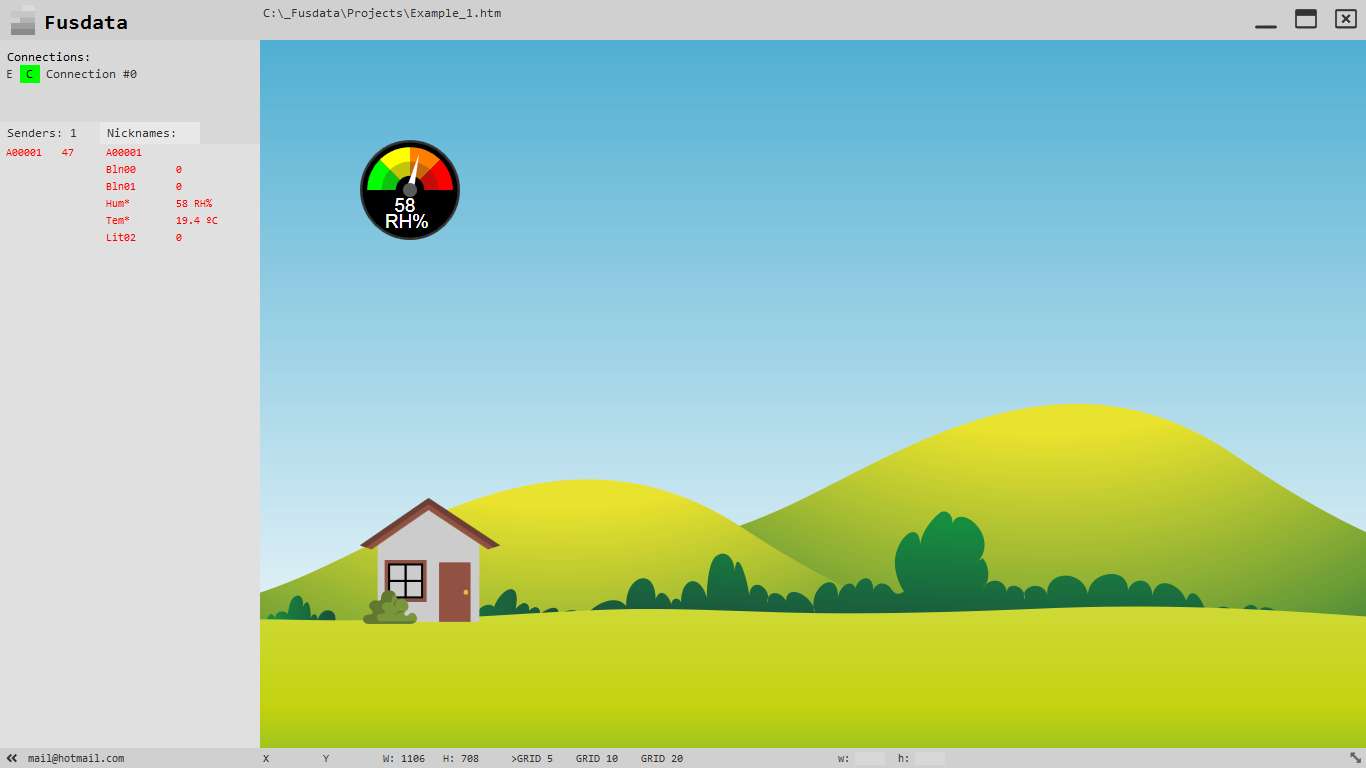
Remenber that you can always change the size and location of each element of the project:
Recuerda que puedes cambiar siempre el tamaño y ubicación de cada elemento del proyecto:
IMPORTANT NOTE:Remember that after modifying any characteristic of a Project you must sabe the changes from the Project menú with “Save” or by pressing CTRL+S.
NOTA IMPORTANTE: Recuerda que luego de modificar cualquier característica de un proyecto debes grabar los cambios desde el menú de proyecto con “Save” o haciendo CTRL+S.
Add an SVG dial to display temperature
Agregar un cuadrante SVG para mostrar la temperatura
Now we should add another SVG graphic to show the temperatura measured by the DHT-11 sensor , for this we proceed the same as in the prevous section, only this time we are choosing another SVG file. Then we add a graphic selecting “Add >” and “SVG Graphic” and a default file will appear again:
Ahora debemos agregar otro gráfico SVG para que se muestre la temperatura medida por el sensor DHT-11, para ello procedemos igual que en el apartado anterior, solo que esta vez vamos a elegir otro archivo SVG. Entonces agregamos un gráfico haciendo “Add >” y “SVG Graphic” y aparecerá nuevamente un archivo default:
First we should choose the new file by clicking on “…” and select the following file:
Primero deberemos elegir el nuevo archivo haciendo click en “…” y elegimos el siguiente archivo:
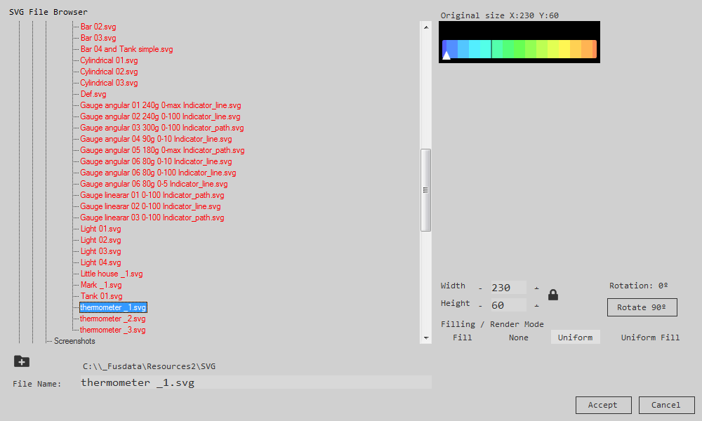
It is located:
C:\_Fusdata\Resources2\SVG\thermometer _1.svg
Then press “Accept” and we can continue modifying the next parameters:
Que se ubica en:
C:\_Fusdata\Resources2\SVG\thermometer _1.svg
Luego de presionar “Accept” podemos seguir modificando los siguientes parámetros:
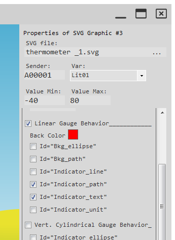
You can see in the figure all the properties to take into account:
SVG file: thermometer _1.svg
Sender: A00001 It is the sender_id of the device that sends the data.
Var: Lit01 It is the “Temperature” variable.
Value Min: -40 Hipothetical value with which the needle points to the minimum.
Value Max: 80 Hipothetical value with which the needle points the scale bottom.
Having selected this file as an SVG graphic, it is defined that we are taljing about a linear dial or “Linear Gauge, that is, just by looking at the shape of the graphic we realice the type of behavoir it will have. That is why we check the “Linear Gauge Behavior” box.
This file does not have internal elements “Bkg_ellipse” or “Bkg_path” because in fact it has a transparent background so we should not check neither box.
Then we can see that the indicator needle is a triangle (it is not a line) so we should check the box “Id=Indicator_path”.
Next we check the “Id=Indicator_text”box so that the graphic shows the numerical value of the temperature.
Se pueden ver en la figura todas las propiedades a tener en cuenta:
SVG file: thermometer _1.svg
Sender: A00001 Es el sender_id del dispositivo que envía el dato.
Var: Lit01 Que es la variable “Temperatura”.
Value Min: -40 Hipotético valor con el que la aguja señala el mínimo.
Value Max: 80 Hipotético valor con el que la aguja señala fondo de escala.
Al haber seleccionado este archivo como gráfico SVG queda definido que estamos hablando de un cuadrante lineal o “Linear Gauge”, o sea, con solo observar la forma del gráfico nos damos cuenta del tipo de comportamiento que tendrá. Por ello marcamos la casilla “Linear Gauge Behavior”.
Este archivo no cuenta con elementos internos “Bkg_ellipse” ni “Bkg_path” porque de hecho tiene un fondo transparente por lo que no debemos marcar ninguna de las dos casillas.
Luego podemos ver que la aguja indicadora es un triángulo (no es una línea) por lo que debemos marcar la casilla “Id=Indicator_path”.
A continuación marcamos la casilla “Id=Indicator_text” para que el gráfico muestre el valor numérico de la temperatura.
Finally, le tus note that this file includes an indication of the “Id=Indicator_unit” box.
It is:
Y por último notemos que este archivo incluye una indicación de la unidad ºC por lo que no debemos marcar la casilla “Id=Indicator_unit”.
Quedará:
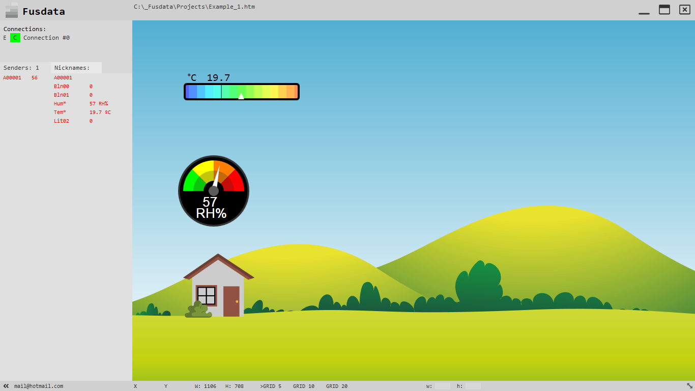
Add a Chart to see the temperature evolution
Agregar un Chart para ver la evolución de la temperatura
Now we propose to add a graphic that shows the evolution of the temperatura in time. For this we have the values of historical records nada n element that can be added to the Fusdata Project, called “Chart”.
To add a new Chart elemet to the Project we have two posible options : we can do it from the Project menú using “Add >” and then “Chart” or we can directly click with the right mouse button on the variable in question in the list of received data from the correponding Sender:
Ahora nos proponemos agregar un gráfico que muestre la evolución de la temperatura en el tiempo. Para ello contamos con los valores de registros históricos y con un elemento que se puede agregar al proyecto de Fusdata llamado “Chart”.
Para agregar un nuevo elemento Chart al proyecto tenemos dos alternativas posibles, podemos hacerlo desde el menú de proyecto mediante “Add >” y luego “Chart” o podemos directamente hacer click con el botón derecho sobre la variable en cuestión en la propia lista de datos recibidos del Sender correspondiente:
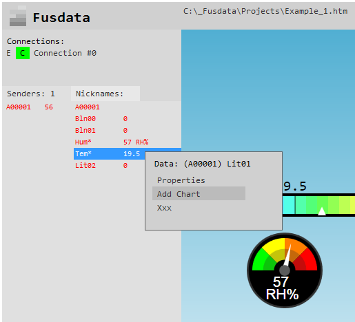
In this way, the chart graphic is added to the Project already linked to the chosen variable.As always, we can now Access the properties of the selected element by clicking on the element itself:
De ésta última manera el gráfico Chart se añade al proyecto ya enlazado a la variable elegida. Como siempre ahora podemos acceder a las propiedades del elemento seleccionado haciendo click sobre el propio elemento:
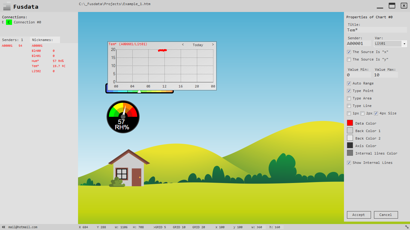
In the properties tab we can make the different settings to modify the behavior and appearance of a chart graphic:
Title: It is the title of the Chart graphic.
Sender: A00001 It is the sender_id of the device that sends the data.
Var: Lit01 It is the “Temperature” variable.
Remember that two historical records can be created, the “x” record that corresponds to the variables as they arrive and the “y” record that also corresponds to the variables that arrive form the Sender devicek, only the original values are replaced by the value recalculated in cas there is a transformation of the corresponding variable.
We should choose chich recordwe want to be displayed on the chart graphic.
Then ifçt should be specified:
Value Min: -40 Hypothetical minimum value to display.
Value Max: 80 Hypothetical maximum value to display.
We can also actívate the “Auto Range”box if we want the graphic to automatically adjust the mínimum and máximum values to be graphed.This option can be very useful but it can cause the chart to look a Little messy.
Then we must choose if we want the graphic to be displayed as a succession of points , afilled área as regards to the X axis, or a series of lines that join the different values. In this regard, it can be said that the “Points” can be more clearly interpreted , taht the “Area” option allows discerning those moments in which there has been a cut in the connection as discontinuities occur , the line option can be useful if we have Little data , but it hide the lack of data.
At the end there are options that allow you to adjust the design and colors of the graphic.
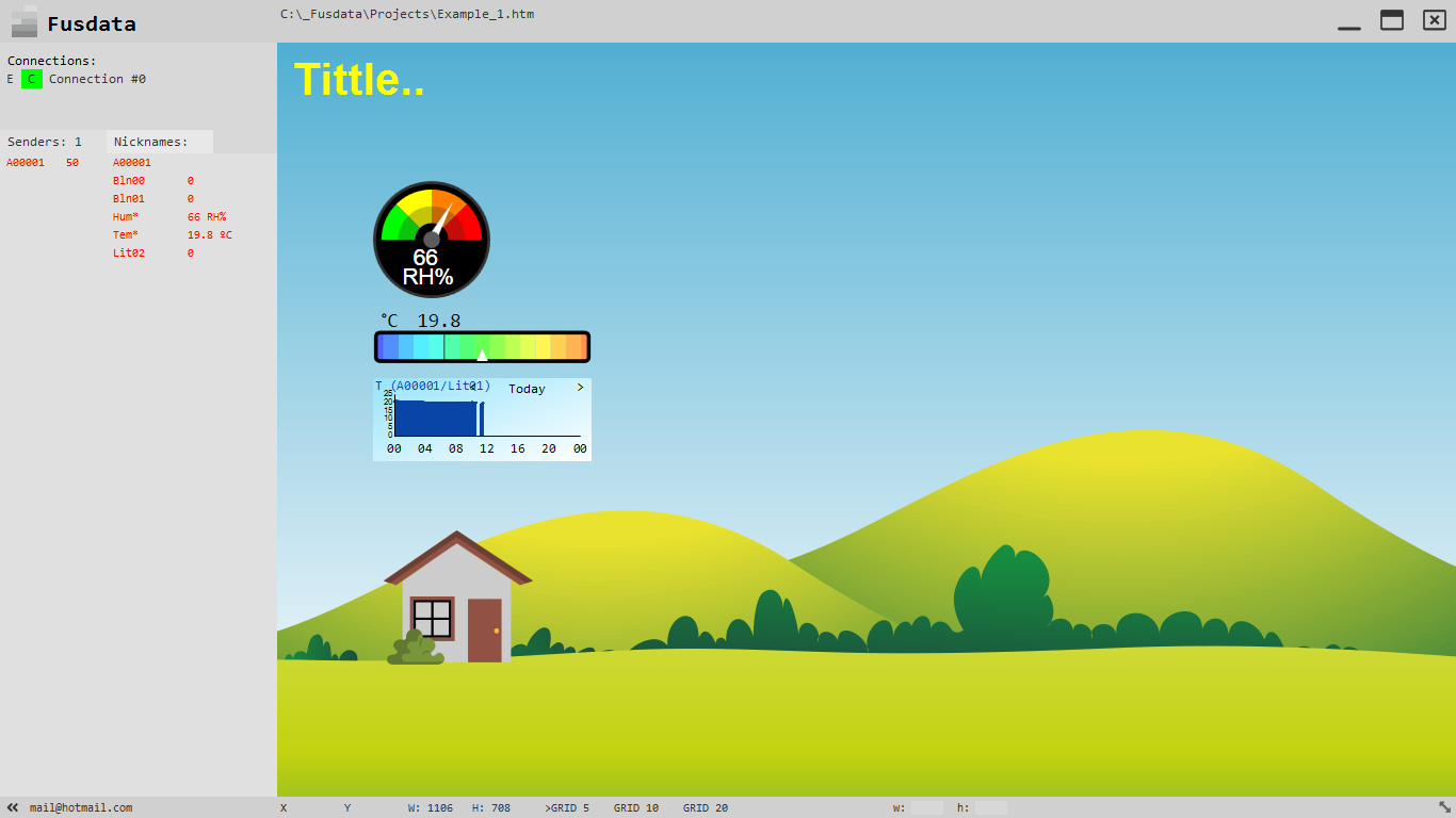
After making all the configurations that we have seen and arraging the elements on the screen bit, I have only added a title using “Add >” and then “Multiline Text”:
En la solapa de propiedades podemos realizar los diferentes ajustes para modificar el comportamiento y la apariencia del gráfico Chart:
Title: Es el título del gráfico Chart.
Sender: A00001 Es el sender_id del dispositivo que envía el dato.
Var: Lit01 Que es la variable “Temperatura”.
Recordemos que se pueden crear dos registros históricos, el registro “x” que corresponde a las variables tal como llegan y el registro “y” que corresponde también a las variables que llegan desde los equipos Sender solo que se remplazan los valores originales por el valor recalculado en el caso de que exista una transformación para la variable correspondiente.
Debemos elegir cual registro deseamos que se muestre en el gráfico Chart.
Luego se especificará:
Value Min: -40 Hipotético valor mínimo a mostrar.
Value Max: 80 Hipotético valor máximo a mostrar.
También podemos activar la casilla “Auto Range” si deseamos que el gráfico se acomode automáticamente a los valores mínimo y máximo que ha de graficar. Esta opción puede ser muy útil, pero puede ocasionar que el gráfico se muestre algo desordenado.
Luego debemos elegir si queremos que el gráfico se muestre como una sucesión de puntos, un área rellena con respecto al eje X o una serie de líneas que unen los diferentes valores. Al respecto se puede decir que la opción “Puntos” puede ser de más clara interpretación, que la opción “Área” permite discernir aquellos momentos en el que se ha producido un corte de la conexión ya que se producen discontinuidades, la opción línea puede ser útil si tenemos pocos datos, pero puede esconder la ausencia de datos.
Al final quedan las opciones que permiten ajustar el diseño y los colores del gráfico.
Después de hacer todas las configuraciones que hemos visto y acomodando un poco los elementos en la pantalla solo he agregado un título mediante “Add >” y luego “Multiline Text” para quedar:
Remember that after modifying any feature of the Project you should sabe the changes from the Project menu using “Save” or by pressing CTRL+S.
Recuerda que luego de modificar cualquier característica de un proyecto debes grabar los cambios desde el menú de proyecto con “Save” o haciendo CTRL+S.
Conclusions
Conclusiones
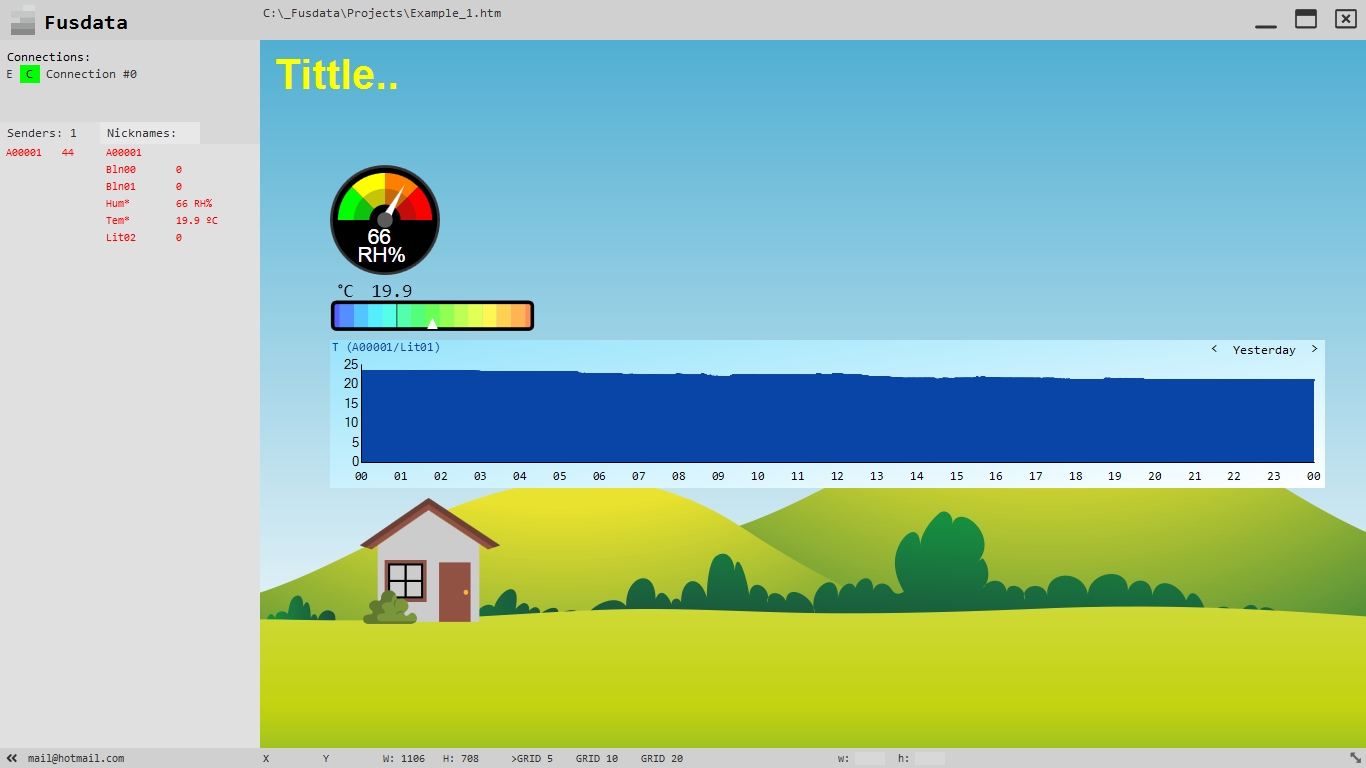
So far we have seen how to set up a simple MQTT telemetry sistema for temperatura and relative humidity inside a house and how to proceed to quicly implement a data presentation screen with Fusdata.
This tutorial has been used to comprehensively visualice the process by which a simple idea becomes a real system.
We can see that after many hours of continous operation, the system has been able to reliably measure, transmit, record ad display the evolution of the RH and temperature variables.
Hasta aquí hemos visto como poner en marcha un simple sistema de telemetría MQTT de temperatura y humedad relativa ambiente dentro de una vivienda y como proceder para implementar rápidamente una pantalla de presentación de los datos con Fusdata.
Este tutorial ha servido para visualizar de manera integral el proceso por el cual una sencilla idea se transforma en un sistema real.
Podemos ver que después de muchas horas de funcionamiento continuo, el sistema ha sido capaz de medir, transmitir, registrar y mostrar la evolución de las variables RH y Temperatura de manera confiable.
It has been posible to verify that the sistema is restored and reconnects tothe Broker when sporadic internet interruptions occur.
The frequency of sendig data for this example has been around 12 seconds, but this value must be reviewed for real applicatins, taking into account the characteristics and the nature of each particular situation, balancing the number samples vs. the resources used.This analysis becomes increasingly importat as the system gets larger.
In my opinión, variables like the ones used in this example could have been monitored with a frequency of the order of the minutes.
As for the quality of the measurement, it can be greatly improved if a DHT-22 sensor is used instead of the DHT-11.
In a future entry I will expose a complete system that will include system of relay outputs and the programming of the connection parametrs in situ.
See you soon my friends.
Diego..
Fusdata.com.ar
info@fusdata.com.ar
Se ha podido comprobar que el sistema se restablece y reconecta al Broker cuando ocurren cortes esporádicos del servicio de acceso a Internet.
La frecuencia de envío de datos para este ejemplo ha sido de alrededor de 12 segundos, pero este valor debe ser revisado para aplicaciones reales, teniendo en cuenta las características y naturaleza de cada situación particular, balanceando cantidad de muestras vs recursos utilizados. Este análisis se hace cada vez más importante a medida que el sistema se agranda.
En mi opinión, variables como las de este ejemplo podrían haber sido monitoreadas con una frecuencia del orden de los minutos.
En cuanto a la calidad de la medición puede mejorar mucho si se utiliza un sensor DHT-22 en lugar del DHT-11.
En una futura entrada voy a exponer un sistema completo que incluirá un sistema de salidas de relé y programación de los parámetros de conexión in situ.
Hasta la próxima amigos.
Diego..
Fusdata.com.ar
info@fusdata.com.ar